Transient Modeling Framework¶

The framework of performing transient simulation using TSNet is shown in Figure 1

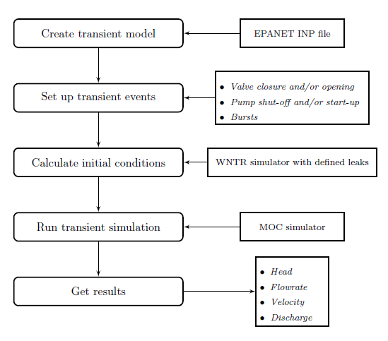
Figure 1 Flowchart of transient simulation in TSNet

The main steps of transient modelling and simulation in TSNet are described in subsequent sections.

Transient Model¶

The transient model inherits the WNTR water network model [WNTRSi], which includes junctions, tanks, reservoirs, pipes, pumps, valves, patterns, curves, controls, sources, simulation options, and node coordinates. It can be built directly from an EPANet INP file. Sections of EPANet INP file that are not compatible with WNTR are described in [WNTRSi].

Compared with WNTR water network model, TSNet transient model adds the features designed specifically for transient simulation, such as spatial discretization, temporal discretization, valve operation rules, pump operation rules, burst opening rules, and storage of time history results. For more information on the water network model, see TransientModel in the API documentation.

A transient model can be created directly from an EPANET INP file. The following example build a transient model.

inp_file = 'examples/networks/Tnet1.inp'
tm = tsnet.network.TransientModel(inp_file)

Initial Conditions¶

TSNet employed WNTR [WNTRSi] for simulating the steady state in the network to establish the initial conditions for the upcoming transient simulations.

WNTRSimulators can be used to run demand-driven (DD) or pressure-dependent demand (PDD) hydraulics simulations, with the capacity of simulating leaks. The default simulation engine is DD. An initial condition simulation can be run using the following code:

t0 = 0. # initialize the simulation at 0 [s]
engine = 'DD' # demand driven simulator
tm = tsnet.simulation.Initializer(tm, t0, engine)

\(t_0\) stands for the time when the initial condition will be calculated. More information on the initializer can be found in the API documentation, under Initializer.

Transient Simulation¶

After the initial conditions are obtained, TSNet adopts the Method of Characteristics (MOC) for solving governing transient flow equations. A transient simulation can be run using the following code:

results_obj = 'Tnet1' # name of the object for saving simulation results
tm = tsnet.simulation.MOCSimulator(tm, results_obj)

The results will be returned to the transient model (tm) object, and then stored in the ‘Tnet1.obj’ file for the easiness of retrieval.

In the following sections, an overview of the solution approaches and boundary conditions is presented, based on the following literature [LAJW99] , [MISI08], [WYSS93].

Governing Equations and Numerical Schemes¶

Mass and Momentum Conservation¶

The transient flow is governed by the mass and momentum conservation equation [WYSS93]:

\[ \begin{align}\begin{aligned}\frac{\partial H}{\partial t} + \frac{a^2}{g} \frac{\partial V}{\partial x} - gV\sin \alpha = 0\\\frac{\partial V}{\partial t} + g\frac{\partial H}{\partial x} + h_f = 0\end{aligned}\end{align} \]

where \(H\) is the head, \(V\) is the flow velocity in the pipe, \(t\) is time, \(a\) is the wave speed, \(g\) is the gravity acceleration, \(\alpha\) is the angle from horizontal, and \(h_f\) represents the head loss (only quasi-steady friction head loss per unit length is modelled in current package).

Method of Characteristics (MOC)¶

The Method of Characteristics (MOC) method is used to solve the system of governing equations above. The essence of MOC is to transform the set of partial differential equations to an equivalent set of ordinary differential equations that apply along specific lines, i.e., characteristics lines (C+ and C-), as shown below [LAJW99]:

\[ \begin{align}\begin{aligned}C+: \frac{dV}{dt} + \frac{g}{a} \frac{dH}{dt} + h_f - gV\sin(\alpha) = 0 \text{ only when } \frac{dx}{dt} = a\\C-: \frac{dV}{dt} - \frac{g}{a} \frac{dH}{dt} + h_f - gV\sin(\alpha) = 0 \text{ only when } \frac{dx}{dt} = -a\end{aligned}\end{align} \]

The explicit MOC technique is then adopted to solve the above systems of equations along the characteristics lines [LAJW99].

Headloss in Pipes¶

TSNet adopts Darcy-Weisbach equation to compute head loss, regardless of the friction method defined in the EPANET .inp file. This package computes Darcy-Weisbach coefficients (\(f\)) based on the head loss (\({h_f}_0\)) and flow velocity (\(V_0\)) in initial condition, using the following equation:

\[f = \frac{{h_f}_0}{(L/D)(V_0^2/2g)}\]

where \(L\) is the pipe length, \(D\) is the pipe diameter, and \(g\) is gravity acceleration.

Subsequently, in transient simulation the headloss (\(h_f\)) is calculated based on the following equation:

\[h_f = f\frac{L}{D}\frac{V^2}{2g}\]

Pressure-driven Demand¶

During the transient simulation in TSNet, the demands are treated as pressure-dependent discharge; thus, the actual demands will vary from the demands defined in the INP file. The actual demands (\(d_{actual}\)) are modeled based on the instantaneous pressure head at the node and the demand discharge coefficients, using the following equation:

\[d_{actual} = k \sqrt{H_p}\]

where \(H_p\) is the pressure head and \(k\) is the demand discharge coefficient, which is calculated from the initial demand (\(d_0\)) and pressure head (\({H_p}_0\)):

\[k = \frac{d_0}{\sqrt{{H_p}_0}}\]

It should be noted that if the pressure head is negative, the demand flow will be treated zero, assuming that a backflow preventer is installed on each node.

Choice of Time Step¶

The determination of time step in MOC is not a trivial task. There are two constraints that have to be satisfied simultaneously:

The Courant’s criterion has to be satisfied for each pipe, indicating the maximum time step allowed in the network transient analysis will be:

\[\Delta t \leqslant \min{\left(\frac{L_i}{N_i a_i}\right)} \text{, } i = 1 \text{, } 2 \text{, ..., } n_p\]

The time step has to be the same for all the pipes in the network, therefore restricting the wave travel time \(\frac{L_i}{N_ia_i}\) to be the same for any computational unit in the network. Nevertheless, this is not realistic in a real network, because different pipe lengths and wave speeds usually cause different wave travel times. Moreover, the number of sections in the \(i^{th}\) pipe (\(N_i\)) has to be an even integer due to the grid configuration in MOC; however, the combination of time step and pipe length is likely to produce non-integer value of \(N_i\), which then requires further adjustment.

This package adopted the wave speed adjustment scheme [WYSS93] to make sure the two criterion stated above are satisfied.

To begin with, the maximum allowed time step (\({\Delta t}_{max}\)) is calculated, assuming there are two computational segments on the shortest pipe:

\[\Delta t_{max} = \min{\left(\frac{L_i}{2a_i}\right)} \text{, } i = 1 \text{, } 2 \text{, ..., } n_p\]

If the user defined time step is greater than \({\Delta t}_{max}\), a fatal error will be raised and the program will be killed; if not, the user defined value will be used as the initial guess for the upcoming adjustment.

dt = 0.1  # time step [s], if not given, use the maximum allowed dt
tf = 60   # simulation period [s]
tm.set_time(tf,dt)

The determination of time step is not straightforward, especially in large networks. Thus, we allow the user to ignore the time step setting, in which case \({\Delta t}_{max}\) will be used as the initial guess for the upcoming adjustment.

After setting the initial time step, the following adjustments will be performed. Firstly, the \(i^{th}\) pipes (\(p_i\)) with length (\(L_i\)) and wave speed (\(a_i\)) will be discretized into (\(N_i\)) segments:

\[N_i = 2\text{int \left(\frac{L_i}{a_i \Delta t\right)} \text{, } i = 1 \text{, } 2 \text{, ..., } n_p\]

Furthermore, the discrepancies introduced by the rounding of \(N_i\) can be compensated by correcting the wave speed (\(a_i\)).

\[\Delta t = \min{\left(\frac{L_i}{a_i(1 \pm \phi_i)N_i}\right)} \text{, } i = 1 \text{, } 2 \text{, ..., } n_p\]

Least squares approximation is then used to determine \(\Delta t\) such that the sum of squares of the wave speed adjustments (\(\sum{{\phi_i}^2}\)) is minimized [MISI08]. Ultimately, an adjusted \(\Delta t\) can be determined and then used in the transient simulation.

It should be noted that even if the user defined time step satisfied the Courant’s criterion, it will still be adjusted.

Boundary Conditions¶

Valve Operations¶

Valve operations, including closure and opening, are supported in TSNet. The default valve shape is gate valve, the valve characteristics curve of which is defined according to [STWV96]. The following examples illustrate how to perform valve operations.

Valve closure can be simulated by defining the valve closure start time (\(ts\)), the operating duration (\(t_c\)), the valve open percentage when the closure is completed (\(se\)), and the closure constant (\(m\)), which characterizes the shape of the closure curve. These parameters essentially define the valve closure curve. For example, the code below will yield the blue curve shown in Figure 2. If the closure constant (\(m\)) is instead set to \(2\), the valve curve will then correspond to the orange curve in Figure 2.

tc = 1 # valve closure period [s]
ts = 0 # valve closure start time [s]
se = 0 # end open percentage [s]
m = 1 # closure constant [dimensionless]
valve_op = [tc,ts,se,m]
tm.valve_closure('VALVE',valve_op)

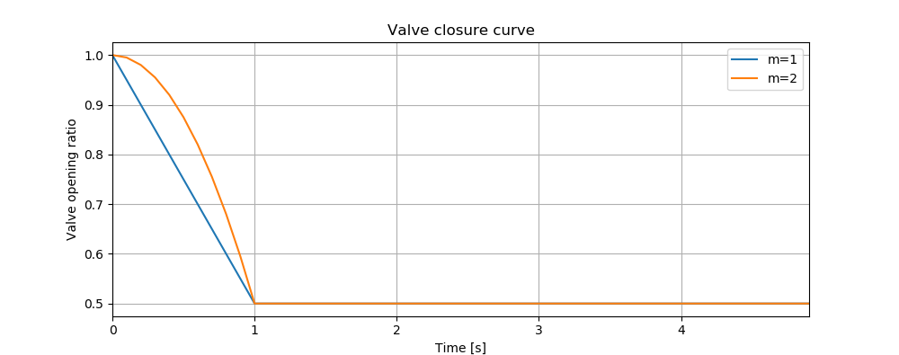
Figure 2 Valve closure operating rule

Furthermore, valve opening can be simulated by defining a similar set of parameters related to the valve opening curve. The valve opening curves with \(m=1\) and \(m=2\) are illustrated in Figure 3.

tc = 1 # valve opening period [s]
ts = 0 # valve opening start time [s]
se = 1 # end open percentage [s]
m = 1 # opening constant [dimensionless]
valve_op = [tc,ts,se,m]
tm.valve_opening('VALVE',valve_op)

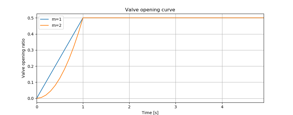
Figure 3 Valve opening operating rule

Pump Operations¶

The TSNet also includes the capability to perform controlled pump operations by specifying how the pump rotation speed changes over time. Explicitly, during pump start-up, the rotational speed of the pump is increased based on the user defined operating rule. The pump is then modeled using the two compatibility equations, a continuity equation, the pump characteristic curve at given rotation speed, and the affinity laws [LAJW99], thus resulting in the rise of pump flowrate and the addition of mechanical energy. Conversely, during pump shut-off, as the rotational speed of the pump decreased according to the user defined operating rule, the pump flowrate and the addition of mechanical energy decline. However, pump shut-off due to power failure, when the reduction of pump rotation speed depends on the characteristics of the pump (such as the rotate moment of inertia), has not been included yet.

The following example shows how to add pump shut-off event to the network, where the parameters are defined in the same manner as in valve closure:

tc = 1 # pump closure period
ts = 0 # pump closure start time
se = 0 # end open percentage
m = 1 # closure constant
pump_op = [tc,ts,se,m]
tm.pump_shut_off('PUMP2', pump_op)

Correspondingly, the controlled pump opening can be simulated using:

tc = 1 # pump opening period [s]
ts = 0 # pump opening start time [s]
se = 1 # end open percentage [s]
m = 1 # opening constant [dimensionless]
pump_op = [tc,ts,se,m]
tm.pump_start_up('PUMP2',pump_op)

It should be noted that a check valve is assumed in each pump, indicating that the reverse flow will be prevented immediately.

Leaks¶

In TSNet, leaks and bursts are assigned to the network nodes. A leak is defined by specifying the leaking node name and the emitter coefficient (\(k_l\)):

emitter_coeff = 0.01 # [ m^3/s/(m H20)^(1/2)]
tm.add_leak('JUNCTION-22', emitter_coeff)

Existing leaks should be included in the initial condition solver (WNTR simulator); thus, it is necessary to define the leaks before calculating the initial conditions. For more information about the inclusion of leaks in steady state calculation, please refer to WNTR documentation [WNTRSi]. During the transient simulation, the leaking node is modeled using the two compatibility equations, a continuity equation, and an orifice equation which quantifies the leak discharge (\(Q_l\)):

\[Q_l = k_l \sqrt{{H_p}_l}\]

where \({H_p}_l\) is the pressure head at the leaking node. Moreover, if the pressure head is negative, the leak discharge will be set to zero, assuming a backflow preventer is installed on the leaking node.

Bursts¶

The simulation of burst and leaks is very similar. They share similar set of governing equations. The only difference is that the burst opening is simulated only during the transient calculation and not included in the initial condition calculation. In other words, using burst, the user can model new and evolving condition, while the leak model simulates an existing leak in the system. In TSNet, the burst is assumed to be developed linearly, indicating that the burst area increases linearly from zero to a size specified by the user during the specified time period. Thus, a burst event can be modeled by defining the start and end time of the burst, and the final emitter coefficient when the burst is fully developed:

ts = 1 # burst start time
tc = 1 # time for burst to fully develop
final_burst_coeff = 0.01 # final burst coeff [ m^3/s/(m H20)^(1/2)]
tm.add_burst('JUNCTION-20', ts, tc, final_burst_coeff)