Example Applications
Example 1 - End-valve closure
This example shows how to simulate the closure of a valve located at the boundary of a network. The first example network is shown below in Figure 12, adopted from [[STWY67],WOLB05]_. It comprises 9 pipes, 8 junctions, one reservoir, 3 closed loops, and one valve located at the downstream end of the system. There are five steps that the user needs to take to run the transient simulation using the TSNet package:
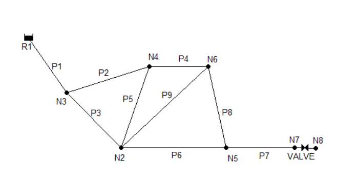
Figure 12 Tnet1 network graphics
- Import TSNet package, read the EPANET INP file, and create transient model object.
import tsnet
# Open an example network and create a transient model
tm = tsnet.network.TransientModel('/Users/luxing/Code/TSNet/examples/networks/Tnet1.inp')
- Set the wave speed for all pipes to \(1200m/s\), time step to \(0.1s\), and simulation period to \(60s\).
tm.set_wavespeed(1200.) # m/s

# Set time options
tf = 20   # simulation period [s]
tm.set_time(tf)
- Set valve operating rules, including how long it takes to close the valve (\(tc\)), when to start close the valve (\(ts\)), the opening percentage when the closure is completed (\(se\)), and the shape of the closure operating curve (\(m\), \(1\) stands for linear closure, \(2\) stands for quadratic closure).
ts = 5 # valve closure start time [s]
tc = 1 # valve closure period [s]
se = 0 # end open percentage [s]
m = 2 # closure constant [dimensionless]
tm.valve_closure('VALVE',[tc,ts,se,m])

# Initialize steady state simulation
- Compute steady state results to establish the initial condition for transient simulation.
tm = tsnet.simulation.Initializer(tm,t0)

# Transient simulation
tm = tsnet.simulation.MOCSimulator(tm)
- Run transient simulation and specify the name of the results file.
# report results
node = ['N2','N3']
tm.plot_node_head(node)
After the transient simulation, the results at nodes and links will be returned and stored in the transient model (tm) instance. The time history of flow rate on the start node of pipe P2 throughout the simulation can be retrieved by:
>>> print(tm.links['P2'].start_node_flowrate)
To plot the head results at N3:
yields Figure 13:

Figure 13 Tnet1 - Head at node N3.
Similarly, to plot the flow rate results in pipe P2:
yields Figure 14:
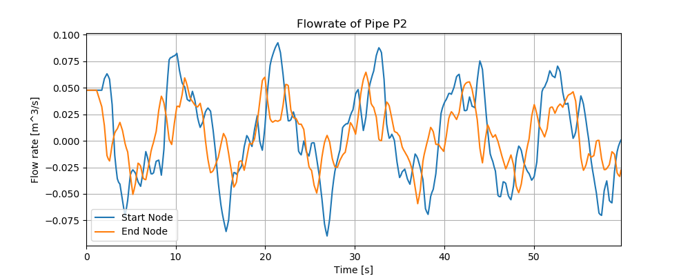
Figure 14 Tnet1 - Flow rate at the start and end node of pipe P2.
Example 2 - Pump operations
This example illustrates how the package models a transient event resulting from a controlled pump shut-off , i.e., the pump speed is ramped down. This example network, Tnet2, is shown below in Figure 15. Tnet2 comprises 113 pipes, 91 junctions, 2 pumps, 2 reservoir, 3 tanks, and one valve located in the middle of the network. A transient simulation of 50 seconds is generated by shutting off PUMP2. There are five steps user needs to take:
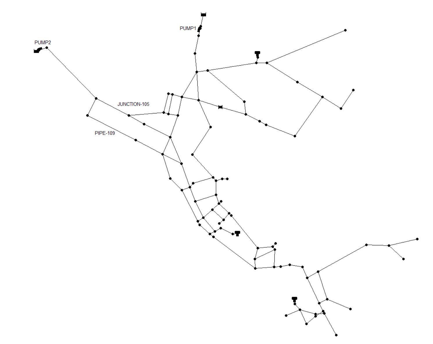
Figure 15 Tnet2 network graphics
- Import TSNet package, read the EPANET INP file, and create transient model object.
import tsnet
# open an example network and create a transient model
inp_file = '/Users/luxing/Code/TSNet/examples/networks/Tnet2.inp'
tm = tsnet.network.TransientModel(inp_file)
- Set the wave speed for all pipes to be \(1200m/s\) and simulation period to be \(50s\). Use suggested time step.
# Set wavespeed
tm.set_wavespeed(1200.)
# Set time step
tf = 20 # simulation period [s]
tm.set_time(tf)
- Set pump operating rules, including how long it takes to shutdown the pump (\(tc\)), when to the shut-off starts (\(ts\)), the pump speed multiplier value when the shut-off is completed (\(se\)), and the shape of the shut-off operation curve (\(m\), \(1\) stands for linear closure, \(2\) stands for quadratic closure).
# Set pump shut off
tc = 1 # pump closure period
ts = 1 # pump closure start time
se = 0 # end open percentage
m = 1 # closure constant
pump_op = [tc,ts,se,m]
tm.pump_shut_off('PUMP2', pump_op)
- Compute steady state results to establish the initial condition for transient simulation.
# Initialize steady state simulation
t0 = 0. # initialize the simulation at 0s
engine = 'DD' # or PPD
tm = tsnet.simulation.Initializer(tm, t0, engine)
- Run transient simulation and specify the name of the results file.
# Transient simulation
results_obj = 'Tnet2' # name of the object for saving simulation results.head
tm = tsnet.simulation.MOCSimulator(tm,results_obj)
After the transient simulation, the results at nodes and links will be returned to the transient model (tm) instance, which is then stored in Tnet2.obj. The actual demand discharge at JUNCTION-105 throughout the simulation can be retrieved by:
>>> print(tm.nodes['JUNCTION-105'].demand_discharge)
To plot the head results at JUNCTION-105:
import matplotlib.pyplot as plt
node = 'JUNCTION-105'
node = tm.get_node(node)
fig = plt.figure(figsize=(10,4), dpi=80, facecolor='w', edgecolor='w')
plt.plot(tm.simulation_timestamps, node._head, 'k', lw=3)
plt.xlim([tm.simulation_timestamps[0],tm.simulation_timestamps[-1]])
# plt.title('Pressure Head at Node %s '%node)
plt.xlabel("Time [s]", fontsize=14)
plt.ylabel("Pressure Head [m]", fontsize=14)


# plt.legend(loc='best')
yields Figure 10:
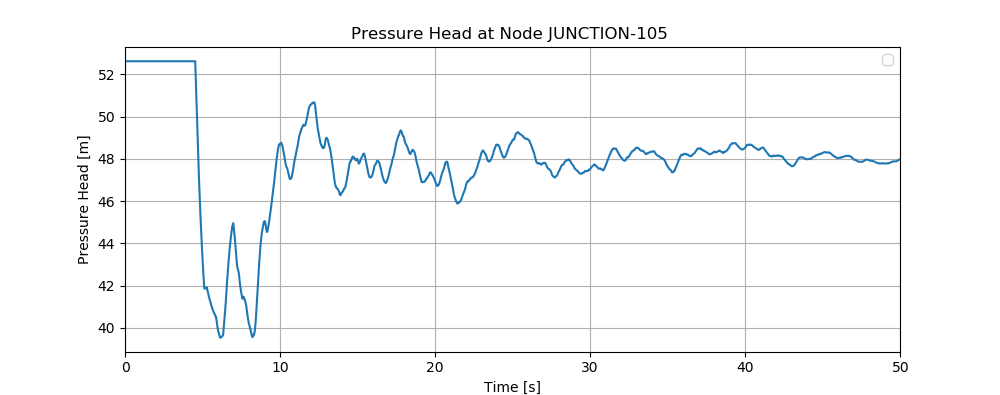
Figure 16 Tnet2 - Head at node JUNCTION-105.
Similarly, to plot the velocity results in PIPE-109:
# fig.savefig('./docs/figures/tnet2_node.png', format='png',dpi=100)

pipe = 'PIPE-109'
pipe = tm.get_link(pipe)
fig = plt.figure(figsize=(10,4), dpi=80, facecolor='w', edgecolor='w')
plt.plot(tm.simulation_timestamps,pipe.start_node_velocity,label='Start Node')
plt.plot(tm.simulation_timestamps,pipe.end_node_velocity,label='End Node')
plt.xlim([tm.simulation_timestamps[0],tm.simulation_timestamps[-1]])
plt.title('Velocity of Pipe %s '%pipe)
plt.xlabel("Time [s]")
plt.ylabel("Velocity [m/s]")
plt.legend(loc='best')
yields Figure 17:
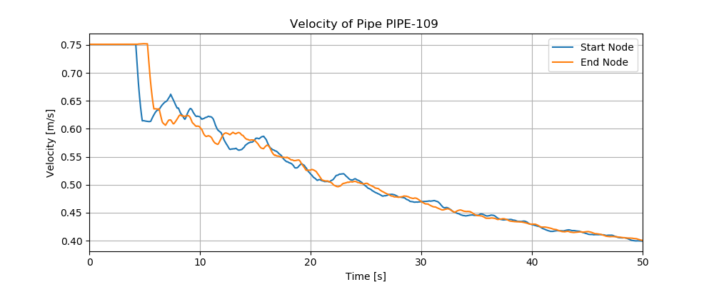
Figure 17 Tnet2 - Velocity at the start and end node of PIPE-109.
Example 3 - Burst and leak
This example reveals how TSNet simulates pipe bursts and leaks. This example network, adapted from [OSBH08], is shown below in Figure 18. Tnet3 comprises 168 pipes, 126 junctions, 8 valve, 2 pumps, one reservoir, and two tanks. The transient event is generated by a burst and a background leak. There are five steps that the user would need to take:
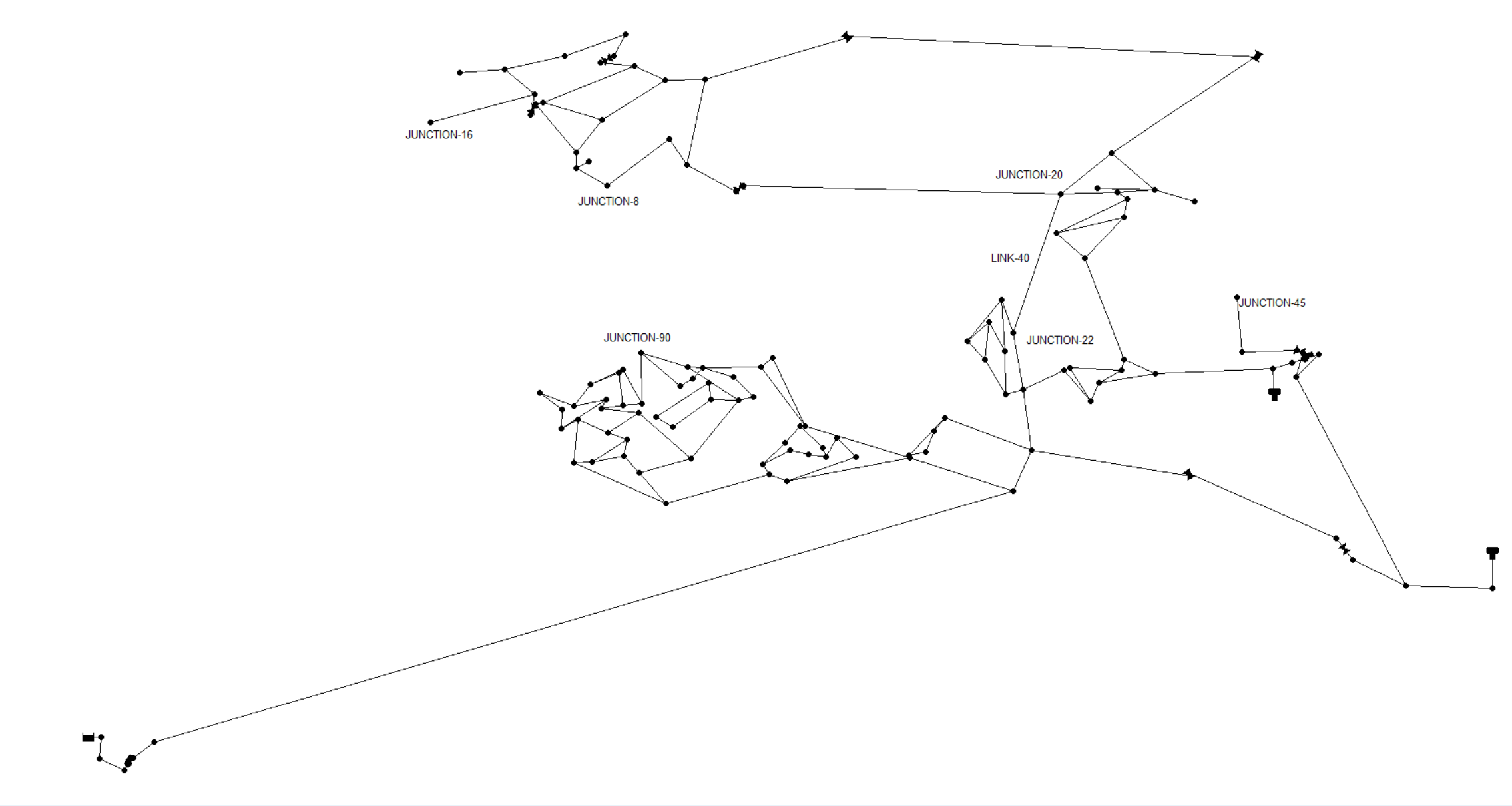
Figure 18 Tnet3 network graphics
- Import TSNet package, read the EPANET INP file, and create transient model object.
import tsnet
# open an example network and create a transient model
inp_file = '/Users/luxing/Code/TSNet/examples/networks/Tnet3.inp'
tm = tsnet.network.TransientModel(inp_file)
- The user can import custom wave speeds for each pipe. To demonstrate how to assign different wave speed, we assume that the wave speed for the pipes is normally distributed with mean of \(1200 m/s\) and standard deviation of :math: 100m/s. Then, assign the randomly generated wave speed to each pipe in the network according to the order the pipes defined in the INP file. Subsequently, set the simulation period as \(20s\), and use suggested time step.
# Set wavespeed
import numpy as np
wavespeed = np.random.normal(1200., 100., size=tm.num_pipes)
tm.set_wavespeed(wavespeed)
# Set time step
tf = 20 # simulation period [s]
tm.set_time(tf)
- Define background leak location, JUNCTION-22, and specify the emitter coefficient. The leak will be included in the initial condition calculation. See WNTR documentation [WNTRSi] for more info about leak simulation.
# Add leak
# emitter_coeff = 0.01 # [ m^3/s/(m H20)^(1/2)]
# tm.add_leak('JUNCTION-22', emitter_coeff)
- Compute steady state results to establish the initial condition for transient simulation.
# Initialize steady state simulation
t0 = 0. # initialize the simulation at 0s
engine = 'PDD' # or Epanet
tm = tsnet.simulation.Initializer(tm, t0, engine)
- Set up burst event, including burst location, JUNCTION-20, burst start time (\(ts\)), time for burst to fully develop (\(tc\)), and the final emitter coefficient (final_burst_coeff).
# Add burst
ts = 1 # burst start time
tc = 1 # time for burst to fully develop
final_burst_coeff = 0.01 # final burst coeff [ m^3/s/(m H20)^(1/2)]
tm.add_burst('JUNCTION-20', ts, tc, final_burst_coeff)
- Run transient simulation and specify the name of the results file.
# Transient simulation
result_obj = 'Tnet3' # name of the object for saving simulation results
tm = tsnet.simulation.MOCSimulator(tm,result_obj)
After the transient simulation, the results at nodes and links will be returned to the transient model (tm) instance, which is subsequently stored in Tnet3.obj.
To understand how much water has been lost through the leakage at JUNCTION-22, we can plot the leak discharge results at JUNCTION-22:
import matplotlib.pyplot as plt
node = 'JUNCTION-22'
node = tm.get_node(node)
fig = plt.figure(figsize=(10,4), dpi=80, facecolor='w', edgecolor='k')
plt.plot(tm.simulation_timestamps,node.emitter_discharge)
plt.xlim([tm.simulation_timestamps[0],tm.simulation_timestamps[-1]])
plt.title('Leak discharge at Node %s '%node)
plt.xlabel("Time [s]")
plt.ylabel("Leak discharge [m^3/s]")
plt.legend(loc='best')
plt.grid(True)
plt.show()
yields Figure 19:
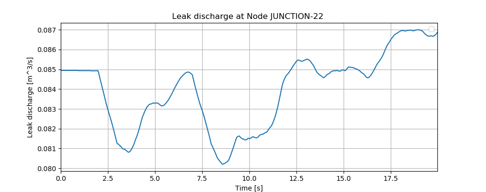
Figure 19 Tnet3 - Leak discharge at node JUNCTION-22.
Similarly, to reveal how much water has been wasted through the burst event at JUNCTION-20, we can plot the burst discharge results at JUNCTION-20:
node = 'JUNCTION-20'
node = tm.get_node(node)
fig = plt.figure(figsize=(10,4), dpi=80, facecolor='w', edgecolor='k')
plt.plot(tm.simulation_timestamps,node.emitter_discharge)
plt.xlim([tm.simulation_timestamps[0],tm.simulation_timestamps[-1]])
plt.title('Burst discharge at Node %s '%node)
plt.xlabel("Time [s]")
plt.ylabel("Burst discharge [m^3/s]")
plt.legend(loc='best')
plt.grid(True)
plt.show()
yields Figure 20:
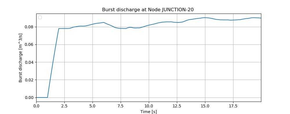
Figure 20 Tnet3 - Burst discharge at node JUNCTION-20.
Additionally, to plot the velocity results in LINK-40:
pipe = 'LINK-40'
pipe = tm.get_link(pipe)
fig = plt.figure(figsize=(10,4), dpi=80, facecolor='w', edgecolor='k')
plt.plot(tm.simulation_timestamps,pipe.start_node_velocity,label='Start Node')
plt.plot(tm.simulation_timestamps,pipe.end_node_velocity,label='End Node')
plt.xlim([tm.simulation_timestamps[0],tm.simulation_timestamps[-1]])
plt.title('Velocity of Pipe %s '%pipe)
plt.xlabel("Time [s]")
plt.ylabel("Velocity [m/s]")
plt.legend(loc='best')
plt.grid(True)
plt.show()
yields Figure 21:
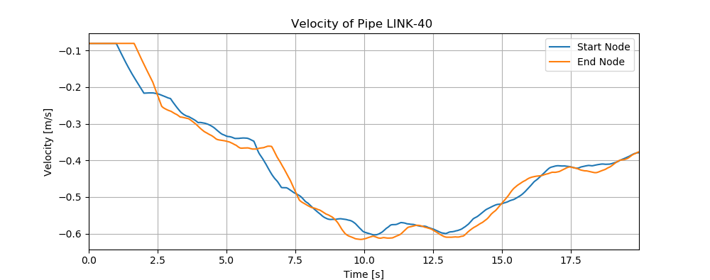
Figure 21 Tnet3 - Velocity at the start and end node of LINK-40.
Moreover, we can plot head results at some further nodes, such as JUNCTION-8, JUNCTION-16, JUNCTION-45, JUNCTION-90, by:
node1 = tm.get_node('JUNCTION-8')
node2 = tm.get_node('JUNCTION-16')
node3 = tm.get_node('JUNCTION-45')
node4 = tm.get_node('JUNCTION-90')
fig = plt.figure(figsize=(10,4), dpi=80, facecolor='w', edgecolor='k')
plt.plot(tm.simulation_timestamps, node1._head, label='JUNCTION-8')
plt.plot(tm.simulation_timestamps, node2._head, label='JUNCTION-16')
plt.plot(tm.simulation_timestamps, node3._head, label='JUNCTION-45')
plt.plot(tm.simulation_timestamps, node4._head, label='JUNCTION-90')
plt.xlim([tm.simulation_timestamps[0],tm.simulation_timestamps[-1]])
plt.title('Head on Junctions')
plt.xlabel("Time [s]")
plt.ylabel("Head [m]")
plt.legend(loc='best')
plt.grid(True)
plt.show()
The results are demonstrated in Figure 22. It can be noticed that the amplitude of the pressure transient at JUNCTION-8 and JUNCTION-16 is greater than that at other two junctions which are further away from JUNCTION-20, where the burst occurred.
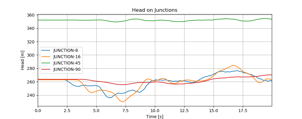
Figure 22 Tnet3 - Head at multiple junctions.
More examples are includeded in https://github.com/glorialulu/TSNet/tree/master/examples.